Abnormality Detection in Chest X-rays (CXR)
Amna Gul, Sheldon Sebastian
Abstract
Keywords: Computer Vision, Deep Learning, Object Detection, Chest X-rays
Video Presentation
Table of Contents:
- Introduction
- Problem Statement
- Problem Elaboration
- Project Scope
- Literature Review
- Methodology
- Data Collection
- Dataset Description
- Exploratory Data Analysis
- Data Preprocessing
- Modeling
- Results & Analysis
- Conclusion
- Project Limitation
- Future Work
- References
- Appendix
Introduction
Problem Statement
Problem Elaboration
Names, as well as class IDs of these abnormalities, are listed below:
| Class Id | Class Name |
|---|---|
| 0 | Aortic enlargement |
| 1 | Atelectasis |
| 2 | Calcification |
| 3 | Cardiomegaly |
| 4 | Consolidation |
| 5 | ILD |
| 6 | Infiltration |
| 7 | Lung Opacity |
| 8 | Nodule/Mass |
| 9 | Other lesions |
| 10 | Pleural effusion |
| 11 | Pleural thickening |
| 12 | Pneumothorax |
| 13 | Pulmonary fibrosis |
Project Scope


Literature Review
Methodology
Data Collection

Dataset Description

The description of each column is given below:
| Column Name | Column Description |
|---|---|
| image_id | unique image identifier |
| class_name | name of abnormality present in a specific image |
| class_id | unique numerical ID (from 0 - 14) assigned to each class in the dataset |
| rad_id | ID of the radiologist (from 1 - 17) that annotated that image |
| x_min, y_min, x_max, y_max |
The last 4 columns contain the bounding box coordinate information for the exact location of the abnormality in an image where (x_min, y_min) tuple represents top left corner and (x_max, y_max) tuple represents bottom right corner of the bounding box. For the “No Finding” class, these columns have NaNs as placeholders. |
A sample image (and its corresponding annotations) from the training dataset is given below:

Exploratory Data Analysis

- 3 of the radiologists (R9, R10, & R8 in that order) are responsible for the vast majority of annotations (~60% of all annotations)
- Among the other 14 radiologists, there is some variation around the number of annotations made, however, these 14 radiologists all made between 3121 annotations and 812 annotations

- Aortic Enlargement is found to be near the aortic vein (above the heart)
- For Cardiomegaly (heart disease), the distribution is concentrated close to bottom corner of the chest
- For all remaining abnormalities, the distribution is lung shaped and relatively diffused


Data Preprocessing
- Converting images from DICOM to png format
- Reducing total dataset size from ~191 GB to ~2.3 GB
- Resizing images as well as their corresponding bounding boxes to 512 x 512 dimension
- Converting single-channel images to RGB channels
- Splitting train data into stratified train-holdout sets (as shown in Figure 8) to evaluate model performance

Modeling
- Resnet152
- VGG19
- Faster RCNN
- YOLOv5
Resnet152 and VGG19:
The final layer had a single neuron that would specify whether the CXR is healthy or unhealthy. The loss function used to train the models was BCEWithLogitsLoss[9]. To handle the class imbalance, the minority unhealthy CXR class was oversampled, and additionally, class weights were used in the loss function[20].
The training data and validation data were normalized using ImageNet statistics. When training the models to avoid overfitting, the following augmentations from the albumentations[21] package were applied for the training dataset:
- RandomBrightnessContrast(p=0.3)
- ShiftScaleRotate(rotate_limit=5, p=0.4)
- HorizontalFlip(p=0.4)
Faster RCNN:
The model was trained for 30 epochs and the model state was saved periodically. The last epoch model was the best performing model. Stochastic gradient descent was used as optimizer with a base learning rate of 0.001. The learning rate scheduler used was warmup cosine and the batch size was 2.
To identify abnormalities of various sizes custom anchor sizes of 2, 4, 8, 16, 32, 64, 128, 256 and 512 were used with aspect ratio of 0.33, 0.5, 1.0, 2.0 and 2.5. The augmentations used for the training dataset are as follows:
- HorizontalFlip(p=0.5)
- RandomBrightnessContrast(p=0.5)
- ShiftScaleRotate(scale_limit=0.15, rotate_limit=0, p=0.5)
YOLOv5:
By default stochastic gradient descent was used as optimizer and the anchor boxes were automatically learned using k-means and genetic algorithm. The learning rate for training was 0.002 and the batch size was 16. The model was trained using the default YOLOv5 data augmentations for a total of 30 epochs.
Ensembling
Ensembling Object Detection Models: To combine the results of Faster RCNN and YOLOv5, weighted boxes fusion(WBF)[5][18] was used with weights of 3:9 respectively. The outputs of Faster RCNN and YOLOv5 were post-processed using NMS with an IoU threshold of 0.3 and a confidence threshold of 0.05. The processed outputs were then fused together using WBF and the fused outputs were again post-processed using NMS with an IoU threshold of 0.3 and a confidence threshold of 0.05
Ensembling Classification and Object Detection Models: We used thresholding logic[19] (as shown in Figure 9) to ensemble the classification and object detection models instead of a hierarchical approach.

In Figure 9, the lower threshold was set to 0.05 and the upper threshold was set to 0.95.
The steps for thresholding logic are as follow:
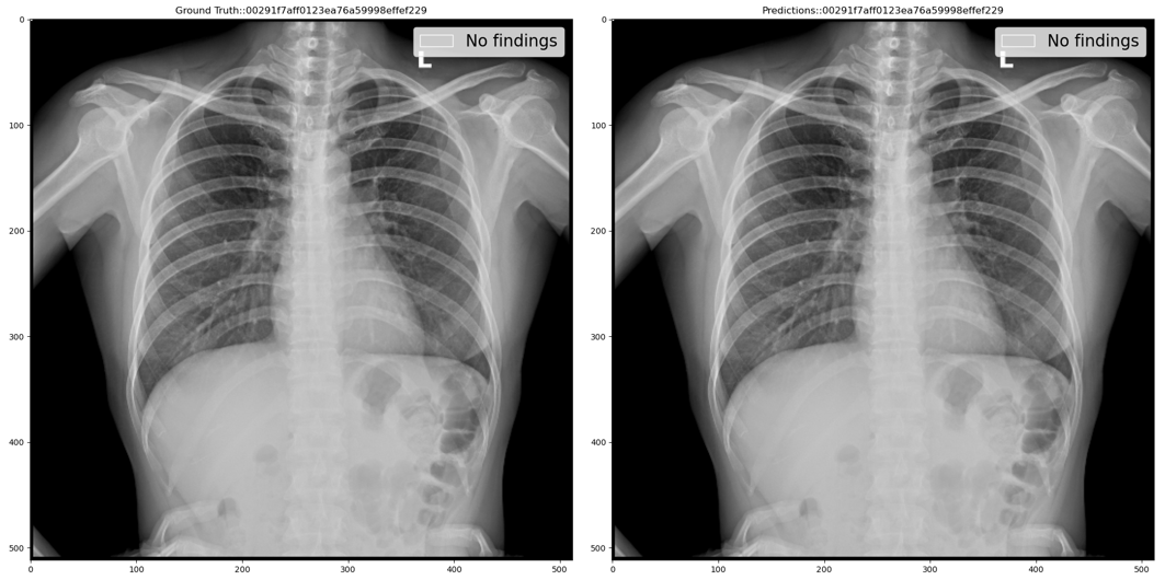
Step 1: If classification model prediction probability (close to 0 means healthy and close to 1 means unhealthy) is less than the lower threshold then use the classification model prediction i.e. No findings class with a 100% confidence score. For example, the below figure shows ground truth vs predicted annotations:
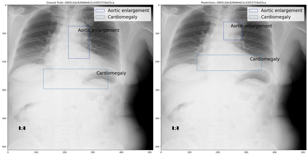
Step 2: If classification model prediction probability is greater than the upper threshold then use the object detection model prediction as is. For example, the below figure shows ground truth vs predicted annotations:
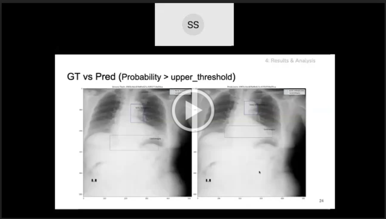
Step 3: If classification model prediction probability is less than the upper threshold but greater than the lower threshold then we add the classification model output i.e. No findings class with classification model prediction probability as confidence score, to the object detection predictions. For example, the below figure shows ground truth vs predicted annotations:
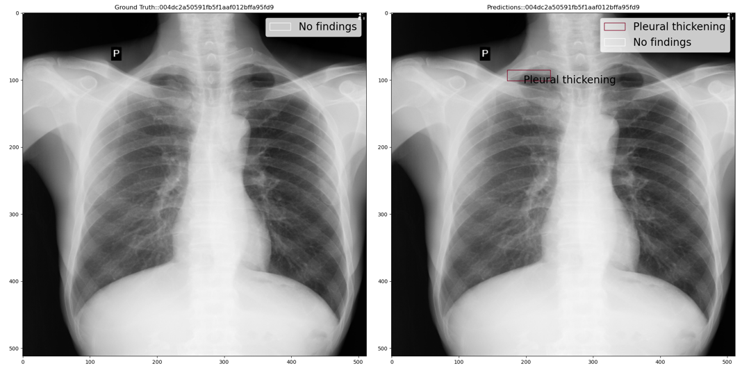
The No Findings class in our dataset is a 1x1 pixel in the top left corner of the image. Thus we need to predict a 1x1 if a chest x-ray is healthy. Using the thresholding logic, mAP of the No Findings class improved from 0.1368 to 0.9582 thus improving the overall mAP from 0.1979 to 0.2903
Results & Analysis
The table below summarizes the individual best performance obtained on each of our deep learning models.

Conclusion
To further validate our results, 3000 test dataset images were passed through our model and final predictions were submitted on Kaggle’s competition page which scored among the top 14% of solutions with mAP of 0.235 on the competition’s private leaderboard.
Based on the results, our model can potentially serve as a second opinion to doctors in diagnosing abnormalities in Chest X-rays. Further improvements in the model can prove to be a stepping stone for automating abnormality detection in Chest X-rays.
Project Limitation
Furthermore, doctors usually consult a patient’s medical history and other demographic metadata before making a prognosis but our dataset did not fully contain that information.
Also, the dataset consisted of 15,000 images which is not a sufficient quantity to fully train a deep learning model for detecting 14 abnormalities. So we tried collecting CXRs from external sources but almost all of the publicly available CXR datasets we found had labels only for classification instead of object detection.
Future Work
- Apply cross-validation techniques on individual models for more robust results
- Performing feature engineering using insights gained from EDA
- Handling class imbalance problem by implementing data augmentation through Generative Adversarial Networks (GANs).
- Deploying our best model on web application e.g. Flask to make it more accessible to the outer world
References
2. Link to EDA Notebook https://www.kaggle.com/guluna/eda-cxr
3. https://www.kaggle.com/sakuraandblackcat/chest-x-ray-knowledges-for-the-14-abnormalities
4. Nguyen, Ha Q., and Khanh Lam et al. VinDr-CXR: An Open Dataset of Chest X-Rays With radiologist’s Annotations. Jan. 2021. https://arxiv.org/pdf/2012.15029.pdf
5. Solovyev, Roman, and Weimin Wang. Weighted Boxes Fusion: Ensembling Boxes for Object Detection Models. Oct. 2019. https://arxiv.org/abs/1910.13302v1
6. Sirazitdinov, Ilyas, et al. “Deep Neural Network Ensemble for Pneumonia Localization from a Large-Scale Chest x-Ray Database.” Computers & Electrical Engineering, vol. 78, Sept. 2019, doi:10.1016/j.compeleceng.2019.08.004. https://www.sciencedirect.com/science/article/abs/pii/S0045790618332890?via=ihub
7. Guo, R., Passi, K.; Jain, C. (2020, August 13). Tuberculosis diagnostics and localization in chest x-rays via deep learning models. https://www.frontiersin.org/articles/10.3389/frai.2020.583427/full
8. https://pytorch.org/tutorials/beginner/finetuning_torchvision_models_tutorial.html
9. https://pytorch.org/docs/stable/generated/torch.nn.BCEWithLogitsLoss.html
10. Yuxin Wu, Alexander Kirillov, Francisco Massa, and Wan-Yen Lo, & Ross Girshick. (2019). Detectron2. https://github.com/facebookresearch/detectron2.
11. https://github.com/facebookresearch/detectron2/blob/master/configs/COCO-Detection/faster_rcnn_R_101_FPN_3x.yaml
12. Wang X, Peng Y, Lu L, Lu Z, Bagheri M, Summers RM. ChestX-ray8: Hospital-scale Chest X-ray Database and Benchmarks on Weakly-Supervised Classification and Localization of Common Thorax Diseases. IEEE CVPR 2017, ChestX-ray8Hospital-ScaleChestCVPR2017_paper.pdf
13. https://detectron2.readthedocs.io/en/latest/modules/data.html?highlight=RepeatFactorTrainingSampler#detectron2.data.samplers.RepeatFactorTrainingSampler
14. https://www.kaggle.com/nih-chest-xrays/data
15. https://www.kaggle.com/guluna/10percent-train-as-test-512images?scriptVersionId=57768659
16. Glenn Jocher, Alex Stoken, Jirka Borovec, NanoCode012, Ayush Chaurasia, TaoXie, … Francisco Ingham. (2021, April 11). ultralytics/yolov5: v5.0 - YOLOv5-P6 1280 models, AWS, Supervise.ly and YouTube integrations (Version v5.0). Zenodo. http://doi.org/10.5281/zenodo.4679653
17. https://github.com/ultralytics/yolov5
18. https://github.com/ZFTurbo/Weighted-Boxes-Fusion
19. https://www.kaggle.com/awsaf49/vinbigdata-2-class-filter
20. Tahira Iqbal, Arslan Shaukat, Usman Akram, Zartasha Mustansar, & Yung-Cheol Byun. (2020). A Hybrid VDV Model for Automatic Diagnosis of Pneumothorax using Class-Imbalanced Chest X-rays Dataset.
21. Buslaev, A., Iglovikov, V., Khvedchenya, E., Parinov, A., Druzhinin, M., & Kalinin, A. (2020). Albumentations: Fast and Flexible Image Augmentations. Information, 11(2).
Appendix
- We tried to merge bounding boxes using Weighted Boxes Fusion at different IoU thresholds to decrease the number of bounding box annotations, but it did not give good results. This could possibly be due to the fact that unmerged bounding box annotations acted as pseudo data augmentation.
- We explored different models such as Resnet50 for classification task and RetinaNet for object detection task, but they did not perform well.
- We preprocessed the CXR images using Contrast Limited Adaptive Histogram Equalization (CLAHE) and Histogram normalization, but they did not give better results and were very computationally expensive.
2. Link to all code files: https://github.com/sheldonsebastian/vbd_cxr
3. Link to download trained model files: https://www.kaggle.com/sheldonsebastian/vbd-cxr-files
